Antipodal Vivaldi Antenna

For a FMCW Radar, a broadband antenna is typically needed. In the example presented here, the bandwidth is only 3%, which could be achieved by several antenna designs. From a practical perspective, the handmade antennas result in a significant variation in antenna center frequency. We have found that the tapered slot [4], or Vivaldi, antenna is an attractive choice, owing to its simplicity to hand-fabricate and very broad bandwidth, which relaxes the need for precise center frequencies. In our design we adopt an antipodal version that will take a microstrip input and transition it to a balanced, tapered slot. Fig. 5 shows the antenna which has been referred by some as a “rabbit ear” antenna, due to the shape of the conductors. It consists of two conductors on either side of a 3.175 mm thick rigid plastic board, commonly used for yard signs, Fig. 5(a). The plastic board is filled with air and thus has a relative dielectric constant of 1. The antenna consists of three parts: 1) a 50 microstrip input, 2) a tapered transition to a parallel trace waveguide and 3) a tapered slot antenna. The fields at the input are between the microstrip and the ground plane of the opposing conductor. As the signal moves outward it slowly transitions to a differential signal between the conductors at the tapered slot.

The design criteria are quite relaxed. The length of Sections 1 and 2 in Fig. 5(a) should be enough to make the transition of the fields smooth. The tapering of the slot line needs only to be a relatively smooth contour, although many papers have attempted to find a mathematically optimal shape, such as a square law shaped design, an exponential shaped design and a simple circular shaped design. The only parameter of relevance is the final width of the taper, which would be a half-wavelength at the largest part. For our design, a 50 microstrip input using the relative dielectric constant of air is 15 mm wide, which sets the initial trace width. Using the target frequency of 925 MHz, the final width is set at approximately 15 cm. The total length is between 1.5 and 2 times the width. The rounded corners of the end assist in making a smooth frequency transition at the lower frequency band.

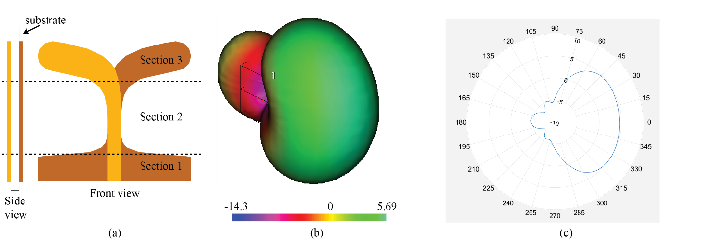Figure 5: (a) Antipodal Vivaldi antenna. Note the different colors represent the top and bottom layers. The three sections of the antenna are marked. (b) Simulated radiation pattern with a peak gain of 5.69 dBi. (c) Polar plot of the measured radiation pattern. The gain is just above 5dBi.

Most antipodal antennas rely on some parameter sweep to optimize their design. In our Radar, we took advantage of NI’s AntSym software, which uses a genetic algorithm to optimize antenna design. We chose only the bandwidth, outline dimensions, and targeted gain (7 dB) and the software optimized the shape. The output design was then imported in to the AWR Axiem software and a full EM simulation was done, which also allowed S-parameter measurements and integration with radio components for simulation. The simulated radiation pattern is shown in Fig. 5(b). The measured antenna pattern is shown in Fig. 5(c). The antenna achieves greater than 10% bandwidth (which is quite small for this type of antenna) and good gain of greater than 5 dBi.

Design

The antenna was designed using Cadence’s Antenna Synthesis Tool, which uses genetic algorithms to find optimal solutions to antenna design problems. The design follows the general guidelines described in the theory section above. For those wanting to explore the antenna, we have provided the design in your template folder: Antipodal_12_17_2019.emp

You can open the file, Window->Tile Vertical and then click the lightening bolt to simulate. You will see the simulation results and field pattern of the radar.

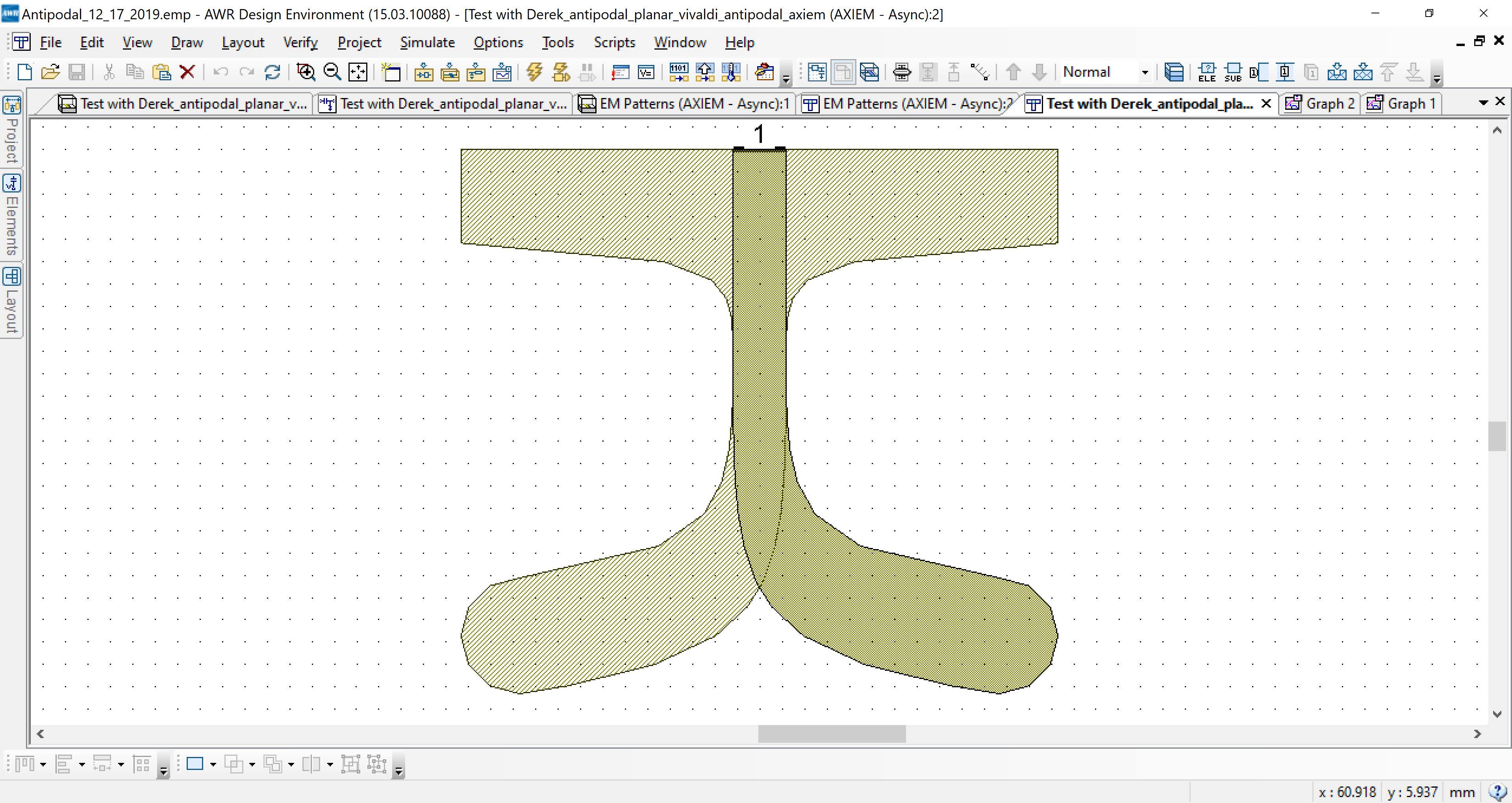
The antenna design was imported from Cadence Antenna Synthesis (AntSyn) software. It generated all of the geometries and dimensions as shown below.

We can take a 3D layout view shown below and see that port 1 is at the input and there is a space between the layers.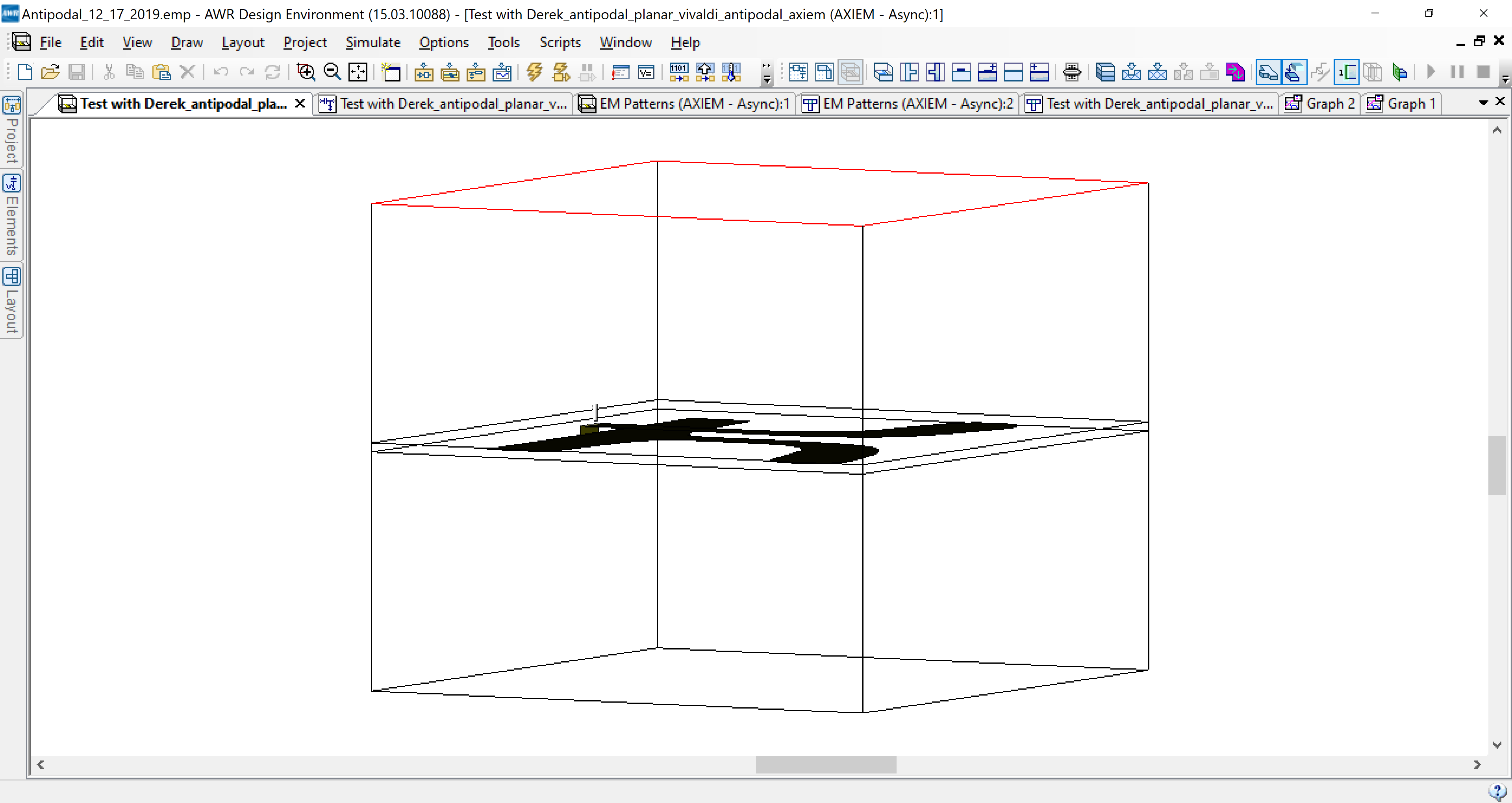

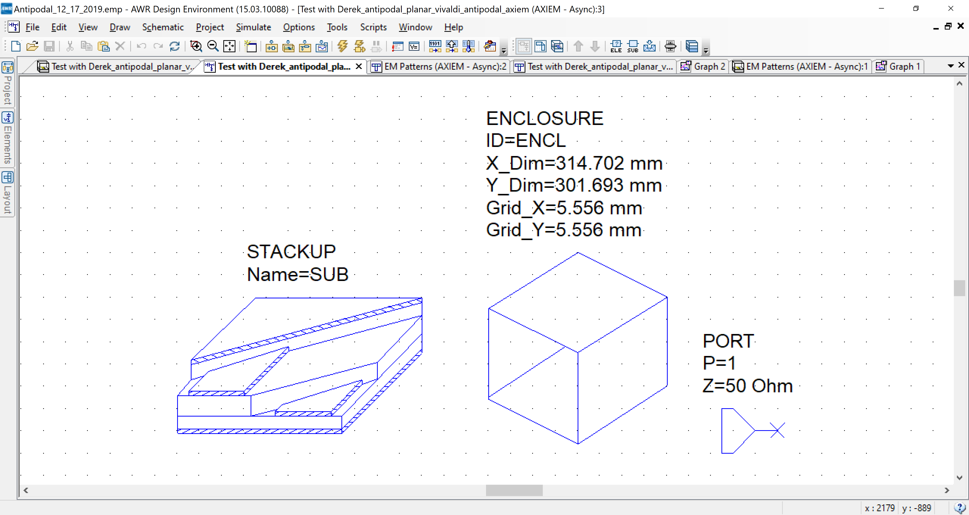
The layout is imported as a EM geometry and enclosure, shown below. The single port, Port 1, is the connection between the traditional circuit simulation and the antenna structure.

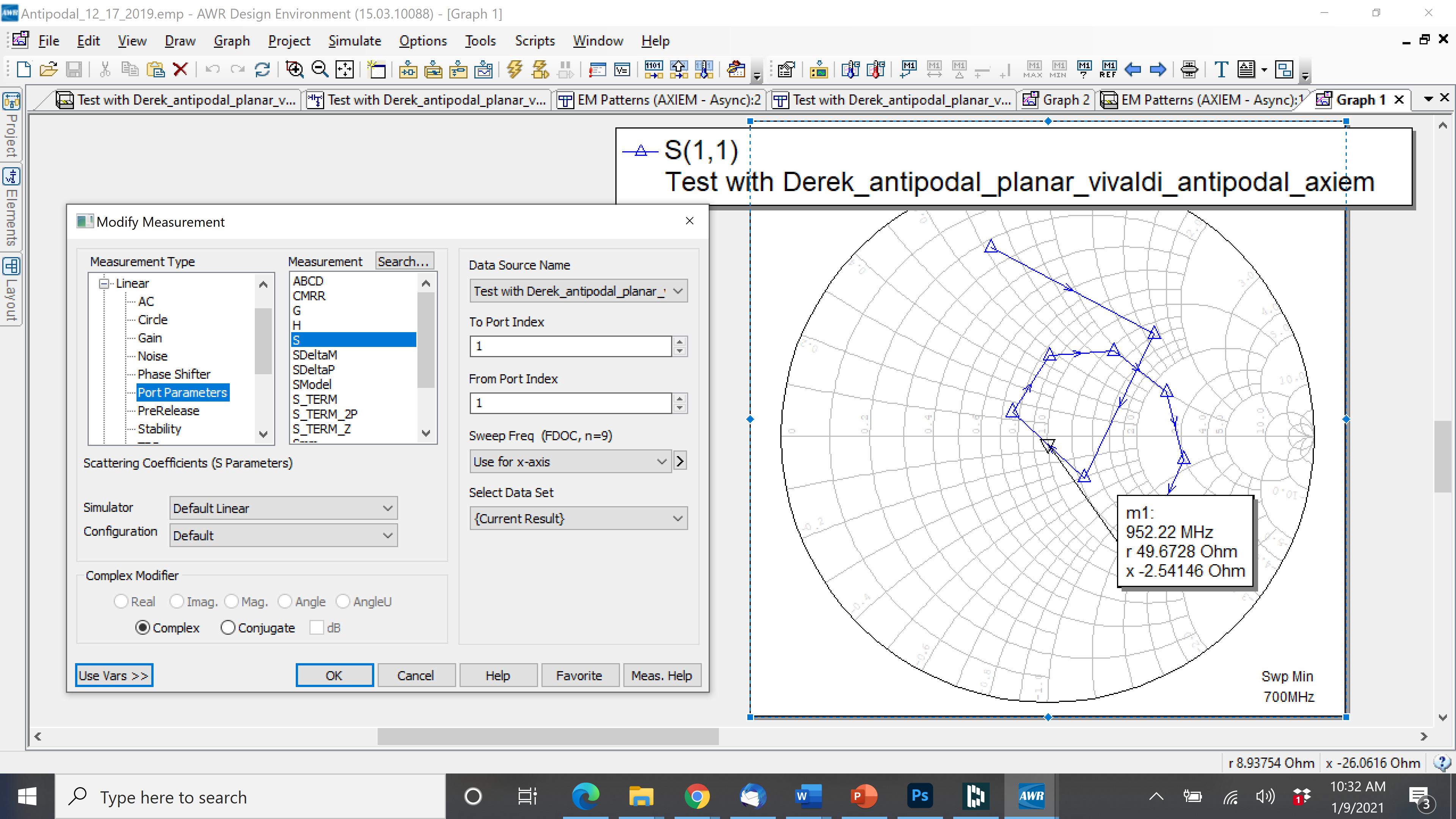
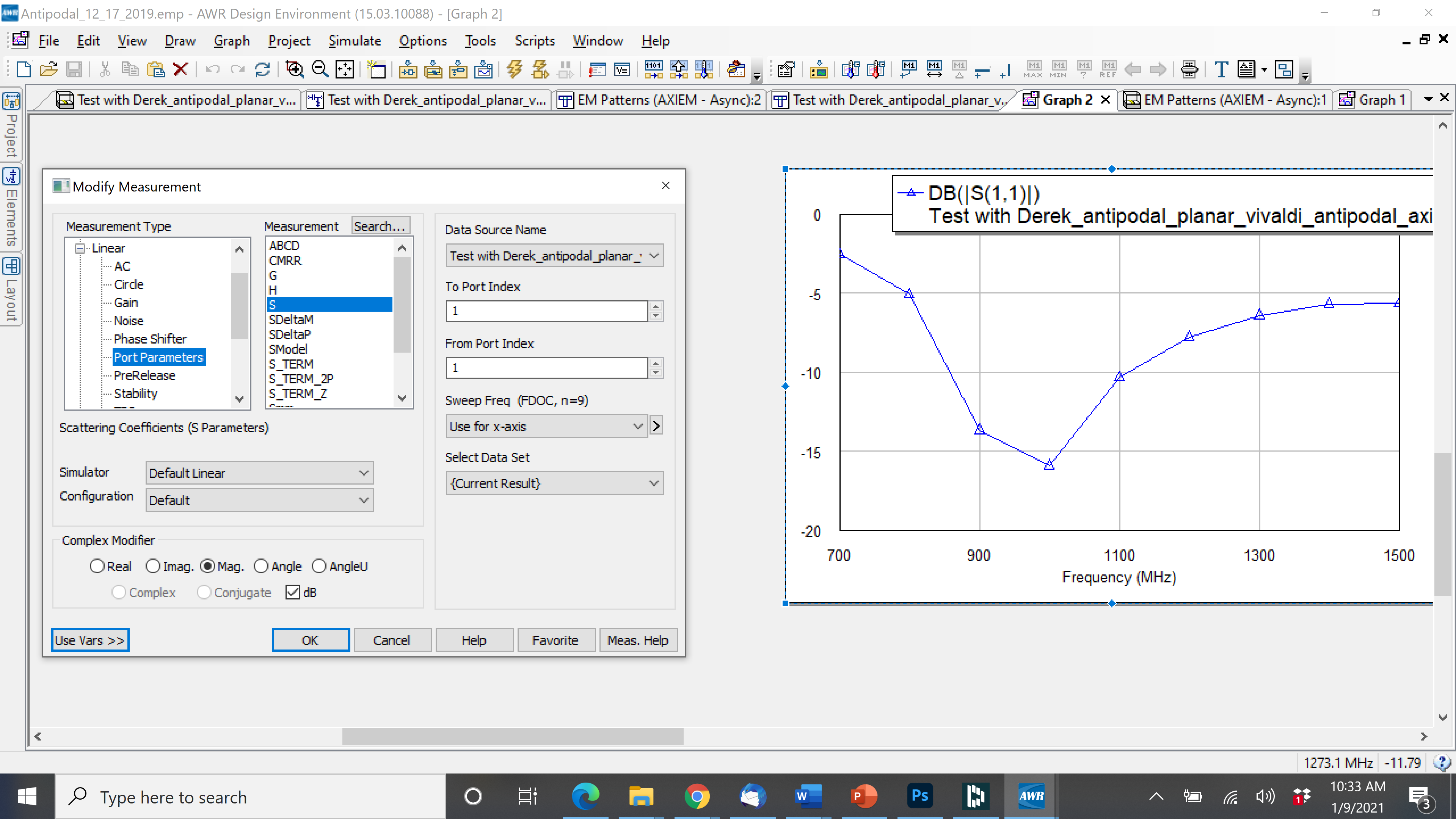
With Port 1 defined, we can plot the complex S11 and S11 dB as we plot any measurement in AWR.

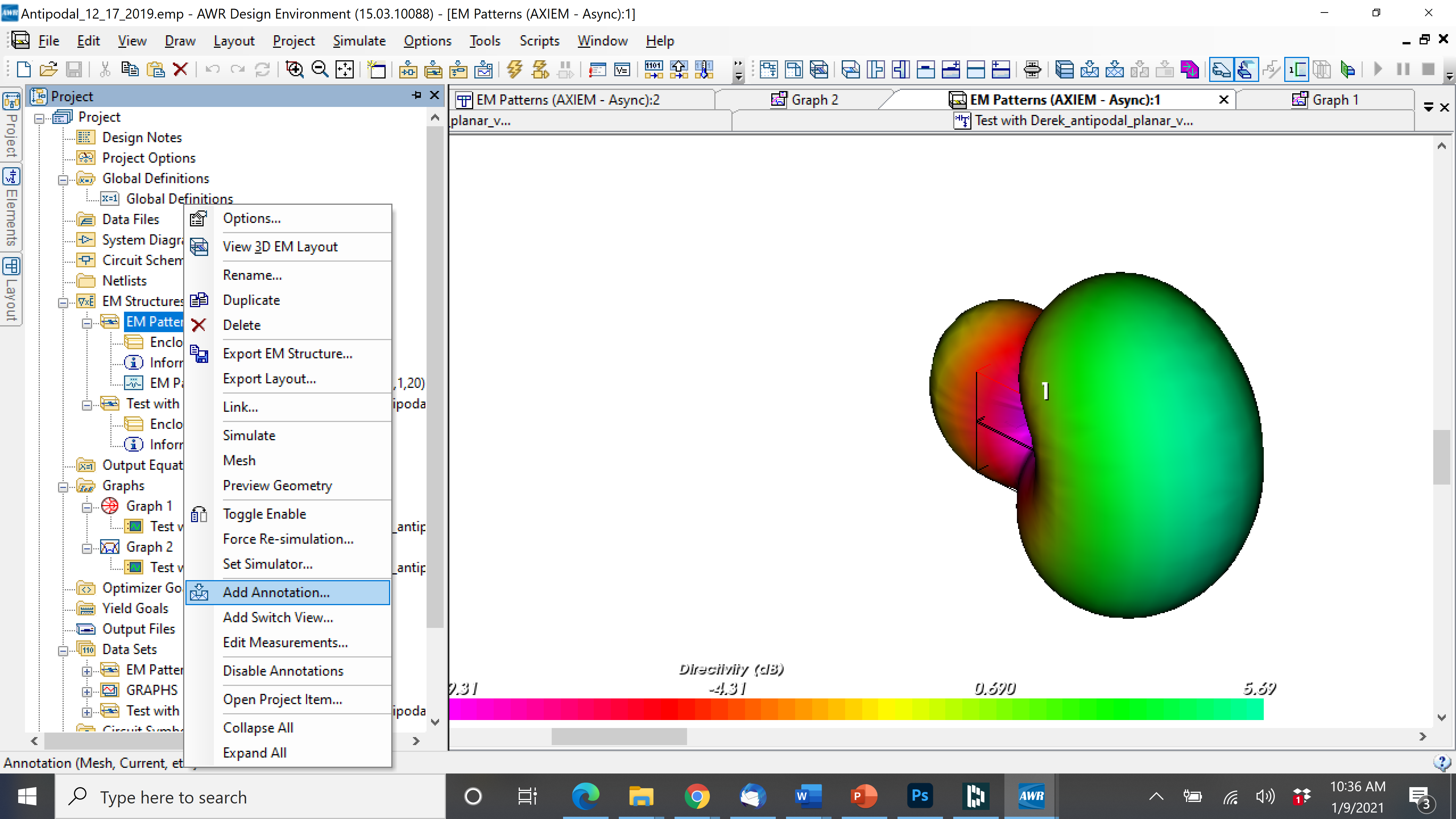
To plot the field patterns, open the Projects tab, go to EM structures->EM Patterns. Right mouse click and select Add Annotation.

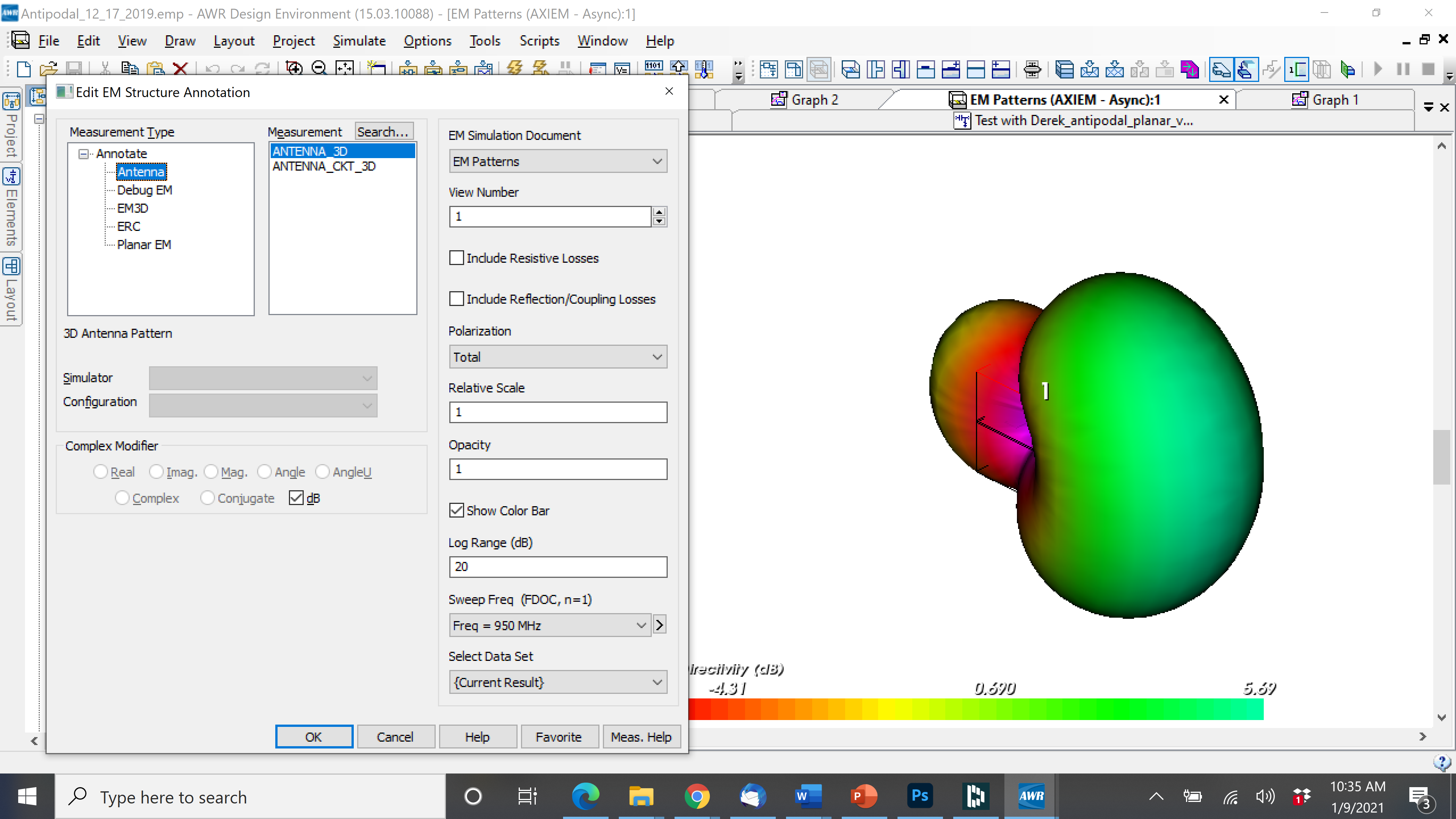
Below are the settings for the Annotation to produce the field plots.

There is no additional design for the antenna, however if you wish to modify the layout, you may and restimulate to see the changes.

Fabrication

To fabricate