
Part 1 – Amplifier Characterization
Load the file Lab 4 – Nonlinearity and Channel Capacity_student_start_v1.emp. Using the Project tab on the left, open the circuit schematic AMP1900 Systems Test. Note, this is a circuit design similar to SPICE you may have done in the past. It is a different schematic type than a System Diagram. The elements in it are from Elements->Circuit Elements, rather than Elements-> System Blocks as we have used in the past. Just note that there is a difference, we will not go further into circuit schematics in his lab. You should see the following amplifier design that includes the transistor level schematic.
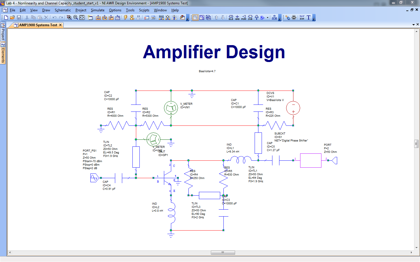
This Circuit Schematic has several parameters/components that are of interest.
- PORT_PS1 – This is an input port that sweeps the power from PStart to Pstep in PStep increments. Its source impedance is 50 ohms.
- PORT – This is a 50 Ohm port that is used both as a termination and as a measurement test point.
The simulator for transistor level circuits can be:
- Time Domain – this simulator steps time in increments and calculates the currents and voltages at each node for each time. This can do full non-linear, time-varying simulations.
- AC Analysis – this simulator finds the dc operating point and linearizes the whole system around that point. It then uses the simplified linear model to perform simulations at one frequency. It can sweep frequencies to give a frequency response. Note: it does not include any nonlinearities. This means that it makes all components “ideal” in a sense. Also, it treats 1e19 Volts the same as 1 mV, to it, they are just numbers in a linear equation; thus there is no physical limitations included.
- Harmonic Balance (HB) – This simulator bridges the gap by performing simulations at several harmonics and pieces together the time domain signals through an inverse Fourier transform. In RF, typically all signals are harmonics of the fundamental so this is an accurate simulation. Typically, 5-9 harmonics are used and can create accurate waveforms in the time domain. AWR defaults to 5 if you do not set other wise. HB performs both linear and nonlinear simulations, with the caveat that the nonlinear behavior is well modeled by the harmonics is simulates.
Setting up the simulation. In AWR you do not explicitly setup the simulator, but do it implicitly through your choice of measurement. When you choose Add Graph-> Add Measurement the measurement you choose selects the simulator for you.
Measurements:
- Linear – AWR will use the AC analysis simulator.
- Nonlinear – AWR will use HB.
- System – Uses VSS time domain, this is a behavioral simulator that simulates in the time domain, but treats all signals just as a complex envelope (the carrier is not considered). This is useful for all of our modulator simulations as we focus on the envelope, not the carrier. The carrier affects on the envelope are included in the simulation. For example, we added phase noise in the past
Go to Options->Project Options->Frequencies. Select the single point box and enter 1.9 (Ghz is implied) and hit Apply. 1.9 should appear on the left. This is the frequency(ies) that AWR will simulate.
To plot waveforms for the amplifier, we will use the Nonlinear Measurement. Below is a screenshot.
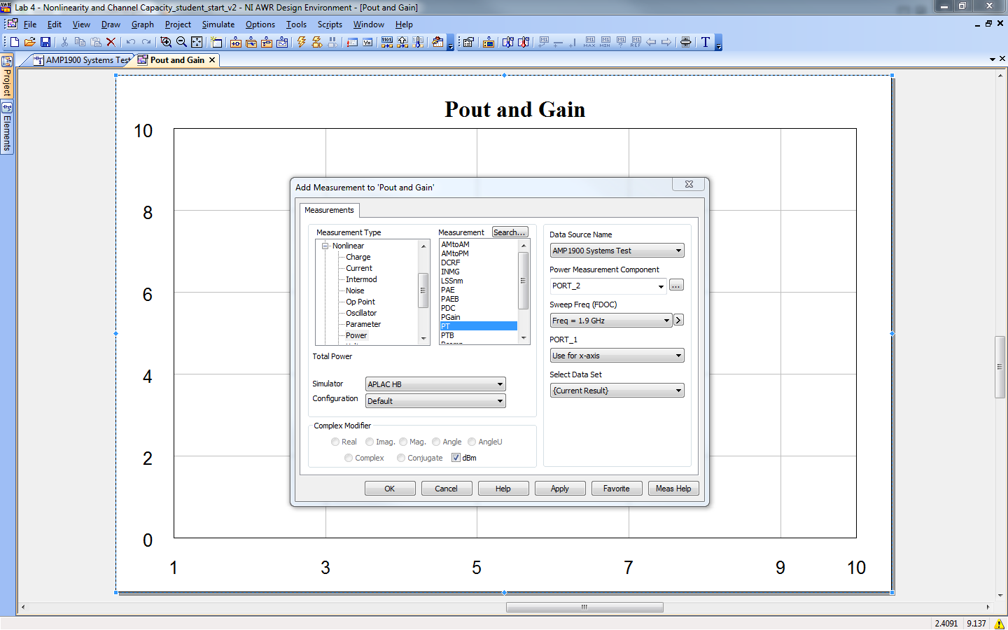
- Measurement Type – Set to Nonlinear-Power
- Measruement –
- PT – Total power at port.
- PGain – Power gain from one port to another (must specify).
- Pcomp – Powerof one harmonic component. You must select harmonic to use.
- Pharm – Powr of all harmonics simulated. In the PORT_1 box you must select on input power, since it is plotting several harmonics (can’t do sweep for multiple signals). HINT: By selecting the slider option in PORT_1 you will plot the first power in the list. Then open the tuner and you can move it to see the results at the other powers. NOTE: The tuner scale is inpoints, i.e. if your power is swept over 16 points, from -32 dBm to 0 dBm by 2 dBm steps, the slider will simply show: 1 to 16. You’ll need to cross reference the actual power.
- Data Source Name – Set to AMP 1900 Systems Test
- PowerMeasurement Component – Set to desired port(s).
- Sweel Freq – Set to 1.9 Ghz (the single freq. you setup).
- PORT_1 – Set to Use for x-axis. NOTE: You have to move the slider UP to see it, the slider default is below this selection, so you don’t see that it is above it.
 For HB and AC simulations there is a fixed length of simulation, so instead of hitting the lightening bold with the play symbol below, push the the single lightening bolt:
Assignment (3 pts):
- Plot the gain and output power of the amplifier. Note the input port sweeps from -70dBm to 0 dBm. Change the Pstop to 20 dBm. Ignore any errors as long as your plot appears.
- What is the power gain of the amplifiers?
- What is the 1dB compression point? Note: use the definition of 1 dB compression point, your knowledge of log-log plots and the marker.
We will now examine the IIP3.
Assignemnt (4 pts):
- Plot Pharm. Select PORT_1 as “Select with tuner.” It will default to the lowest power.
- Using the tuner, change the input power from level 6 to step 7 (note that the power sweep is in 2 dBm increments, so one step change is 2 dB input power change). What is the change in the power of each harmonics.
- Comment on the trend and any discrepancies from what you would expect
- Using Pcomp, plot the 1st and 3rd harmonics vs. input power. Graphically, calculate the IIP3 point. Note: you may want to paste in the plot and use a line in word to draw and find the intercept graphically.
Part 2 – Spectral Growth
Open the 16QAM System diagram. It should look like the screen shot below:
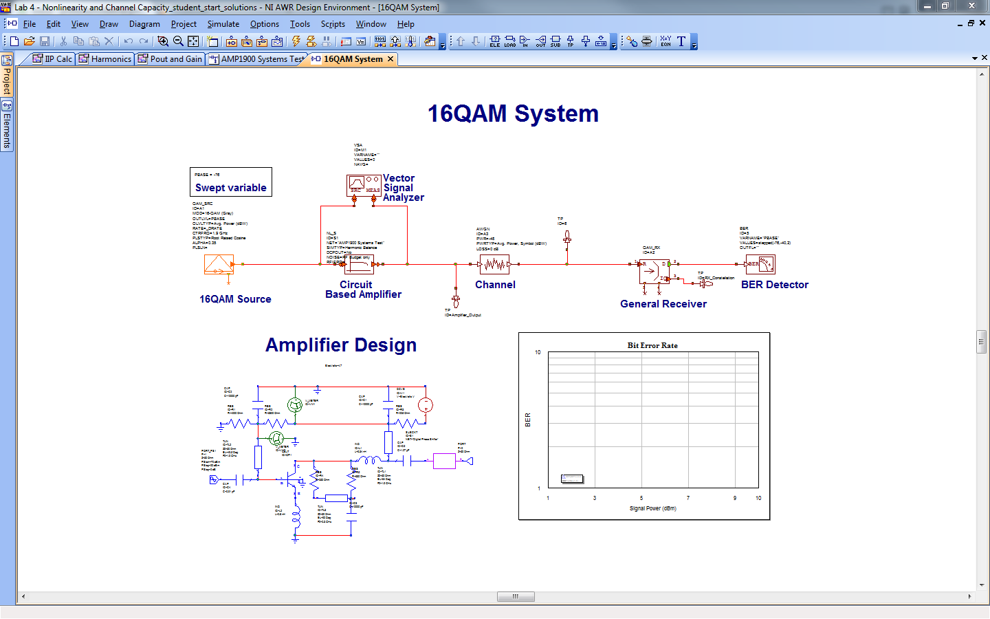
It consists of the following:
- QAM_SRC – This is an idealized QAM source that creates the I and Q signals on the Re and Im components of its complex output.
- MOD – modulation order
- OUTLVL – Output power level – it is set to a variable PBASE.
- _DRATE – It inherits the System Default Options for symbol rate. It is 1 MS/s in this system.
- CTRFRQ – Center frequency of the system. This is needed because the amplifier is a circuit schematic so it has to do that simulation in HB which requires the frequency components of the input.
- PLSTYPW – Filter type.
- ALPHA – alpha of filter.
- NL_S – this is a symbol for the amplifier sub-circuit.
- VSA – Used for measurements (not in this lab).
- AWGN – Additive White Gaussian Noise.
- PWR – sets noise power. -48dBm in this lab.
- LOSS – sets any signal attenuation through the channel. 0 dBm in this lab (no loss).
- QAM_RX – Behavioral receiver for QAM. NOTE: It “talks” to the QAM_SRC to coordinate modulation order symbol rate, etc.
- D – is the data as numbers.
- IQ – is complex signal: I is Re and Q is Im.
- BER – Bit error-rate. It tells you how many bits can be received before you have an error, on average. The detector is setup to sweep something and measure the BER vs. that parameters. In this lab it is PBASEb which is the input power. It could be the noise power, SNR, or several other useful parameters.
- VARNAME – The variable it will sweep.
- VALUES – The values for the sweep. -76 dBm to -40 dBm in 2 dBm steps in this lab.
To simulate this system, you select the usually lightening bolt with the play button below.
Assignment(2 pts):
- Plot the spectrum of the amplifier output. Run the simulation. What happens qualitatively to the level and shape? You do not need to place a plot here as it changes. Answer in text only.
- Explain the change in amplitude. Explain the change in shape.
Part 3 – Channel
We will examine the channel through the following questions. Change your filter to Raised Cosine.
We will start by examining the relationship between symbol rate, bit rate and bandwidth.
Assignment(4 pts):
- Using your FFT from the previous assignment. What is the BW of this signal? It may be helpful to change the axis of the FFT to see the venter better. BW is defined as the BW at 3dB below the peak.
- What should the theoretical BW be? If it differs from the number above, please explain.
- Change the modulation order to 64 QAM. Does the BW change? Explain why/why not.
- What is the bit rate at 16 QAM and now at 64 QAM?
Now let us look at the channel.
Assignment(2 pts):
- Plot the FFT of the output of the AWGN block as well as the output of the amplifier on the same FFT. This is your signal from the amplifier after it has passed through a noisy channel (noise was added). Paste the final FFT below. Describe what qualitatively happened as the input power increased.
- Why is the shape after the channel different than at the output of the amplifier? Why is it that shape?
Now let us look at the receiver. Reset your QAM to 16. Set your filter to Rectangular.
Assignment(7 pts):
- Plot the wavform at D and the constellation at IQ after the QAM_RX block. NOTE: Hit pause when the constellation appears and paste that waveform in along with D. What format is D in?
- Why does the constellation not appear right away? Hint: what is changing during the simulation (both input and in the channel).
- From the Project tab, you can double click on the Bit Error Rate plot to make it visible. Run the simulation. The BER tells you 1/(# of good bits) on average. So a BER of .001 means you get, on average, 1000 goo bits before an error. Plot the BER below.
- Explain why it reduces initially with signal power and then increases?
- Change to a Root Raised Cosine filter (the receiver has the other half of the raised cosine)? Plot the BER. Does the BER change – if so why?
- Change your modulation to 64 QAM? Plot the BER. Does it change and how?
- Explain why the BER changes? HINT: Look quantitatively at the constellation of the Rx. Set the noise to -100 dBm to see it for 64 QAM
Assignment(3 pts):
- Calculate C. Do this in excel or similar. Use B=500kHz*1.35=675 kHz? You have the noise power for the AWGN, you know the range of signal power from the amplifier gain and/or measurements. Make sure you keep track of dB and/or linear.
- Is your does your experimental results match with your C? Are you exceeding the limit? Are you below the limit?
- Using C and the given noise of your system, what is the maximum useful M? (meaning a larger M does not bring any benefit).
Comments are closed.