
Part 1 – I/Q Imbalance
Load the file QAM_w_Phase_Noise_&_Imbalance.emp. The System Diagram should look like the one below. Watch the video “QAM System Simulation with Imbalance and Noise” to understand how the block diagram works.
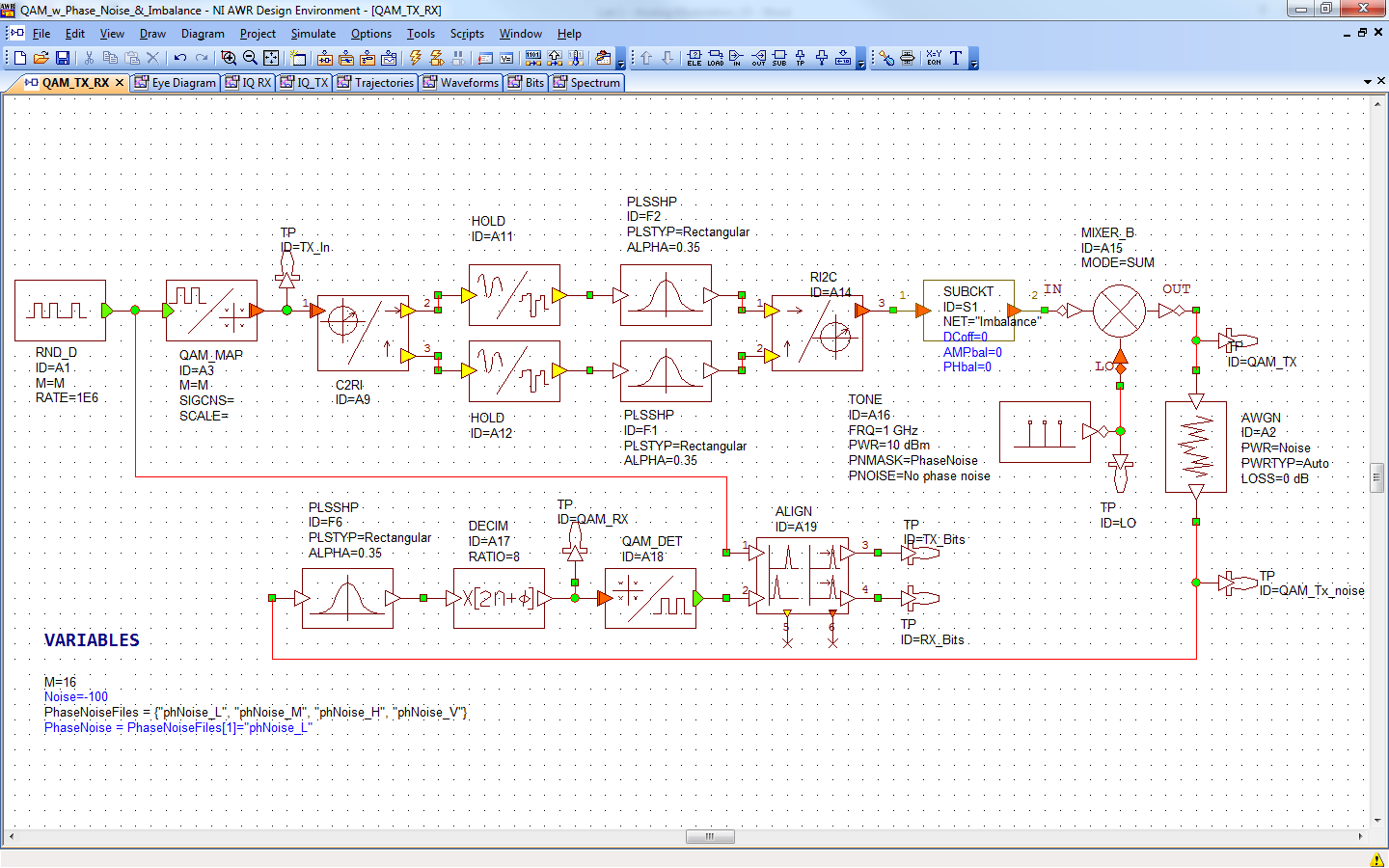
Explore each block to see the settings – they are not listed explicitly in this document since you have the file to reference.
This System Diagram has several parameters that can be adjusted.
There are 5 tunable parameters – set these to the values shown below to start.
- DCoff=0– the DC offset/imbalance in the I/Q path.
- AMPbal=0 – the amplitude imbalance in the I/Q path.
- PHbal=0 – the phase imbalance in the I/Q path.
- Noise=-100 – the level of added noise in the AWGN – additive white noise block.
- PhaseNoise=1 on tuning slider– the phase noise spectrum of the LO. Four phase noise profiles have been added to the project. In the Project browser, select Data Files and you will see hich file. Double click to see how they are organized. It gives pairs of frequencies and noise levels that map out the spectrum of the oscillator. Note the frequencies are offset frequencies form the carrier, not absolute frequencies.
There are two menu driven parameters
- Chg_PLSSHP_Filter=Rectangular –(NOTE: This changes multiple blocks in the System Diagram, so should be used for changing filter types) – this is found by selecting QAM_TX_RX as the active window. Then from the menus at the top of the AWR: Scripts->ProjectScripts-> Chg_PLSSHP_Filter. This brings up a menu of different filter types. Note that it defaults to the Root Raised Cosine when opened, regardless of what the filter was set at before, i.e. you can’t “check” what the filter is by going to the script. Rather, you need to look at PLSTYP of the PLSSHP filter block.
- Toggle_phNoise=OFF – this turns ON and OFF the phase noise of the LO. It can be found in the same ProjectScripts as the Chg_PLSSHP_Filter. You can see the state by looking at the TONE block that is the LO and examining PNOISE. It will say No phase noise or Generate phase noise. The phase noise spectrum used is defined by PNMASK=PhaseNoise, where we have made PhaseNoise a variable that goes from low (Level 1) to high (level 4) noise. You can directly change this by clicking on PNOISE and using the drop-down menu that appears.
Using the script function, make sure all filters are “Rectangular”. Run the simulation and then pause. Make sure the filters are set to rectangular and phase noise is off.
Assignment (5 pts):
- Plot the waveforms of the real and imaginary parts of QAM_TX and QAM_TX_noise on two separate Left axis. Comment on any difference.
- Plot the eyediagrams for the QAM_TX_noise, placing I and Q on separated Left axis.
- Plot the IQ diagram for QAM_TX and QAM_TX_noise on one IQ plot and also QAM_RX on a separate graphs. It will be helpful to set the limits for the QAM_Tx plot to 0.6 and the limits on the QAM_Rx to 1.4, with divisions set to 0.3 and 0.7 respectively. This will keep the axis fixed as we change things later.
- Plot the Spectrum of (make sure to select dB scale): The LO, Qam_Tx and QAM_Tx_Noise. For QAM_Tx_Noise, add a symbol at an interval of 25 and size of 3 – this will aid in seeing it when it is on top of QAM_TX. Comment on the difference between the QAM_Tx and QAM_Tx_Noise.
- Plot the waveforms of TX_Bits and RX_Bits on the same plot. Choose 40 Symbols as the Time Span. These are a received and decoded version of the bits. The TX_Bits is derived from the transmitter and used to synchronize the receiver. Also, the received Symbol is decoded into the multilevel signal generated by the RND_D block with M=16. Add a circular symbol to the RX_Bits with the interval set to 1 (that is 1 Symbol since the bits are decoded into Symbols by QAM_DET).
Open up the tuner bar. In the following, tune the parameter mentioned and examine its affect.
Assignment (4 pts):
- Plot the IQ_TX (with and w/o noise – same plot) and then plot the wavforms for an Amplitude imbalance of 5. (Two plots total) Describe what has changed in the IQ and in the waveforms.
- Plot the IQ_TX (with and w/o noise – same plot) and the wavform for an DC offset of 0.2. Describe what has changed in the IQ and in the waveforms.
- Plot the IQ_TX (with and w/o noise – same plot) and the wavform for phase shift of 45 degrees. Describe what has changed in the IQ and in the waveforms. How many levels does I and Q have with the phase shift?
- Plot the eye diagram for phase shift of 45 degrees. Describe what has changed from zero phase shift. How many levels does I and Q have with the phase shift? (its easier to see in the eye diagram).
Reset all of the imbalances to zero. Now view the Bits graph. When you are receiving the same signal as is being transmitted, the RX_Bits and TX_Bits waveforms will overlap. The symbol you added on the RX_Bits helps you see this. Below, you are going to adjust each parameter until one bit of RX_Bits differs from the TX_Bits. This would be a Bit Error Rate (BER)[1] of 1 per 40 Symbols, or .025, which is VERY high. Typical systems are 10-6 or below, e.g. 10-9. Note: You can set the decimal number for the parameter in the tuner window by typing it in the top box. This gives you more precision than with the mouse. You can also set the resolution of the tuner with the bottom box.
Assignment (5 pts):
- Adjust the DC offset until one (or a few) bit is incorrect in the plot. Paste the Bits waveform below. What was the DC offset?
- Set the DC offset to zero and paste in the IQ_RX plot below. Measure the I axis values for each column and report those values. These represent the center of the constellation. The receiver draws an imaginary box around those center points, that separates two adjacent point evenly. Given the numbers you found where would the decision boundary be for the I axis, e.g. if the left most column moved to the right along the I-axis, at what value would it be considered to be in the nominal second from the left columns area or box.
- Now set the DC offset to the value that caused the first bit errors. What is the I value of the left most column? Is that consistent with your answer above, i.e. was your predicted decision threshold value the same as when the errors started in the RX_Bits plto? Plot the IQ_RX constellation with a marker to show the decision.
- What is the Amplitude imbalance for the first bit errors? (just give number)
- What is the Phase imbalance for the first bit errors? (just give number)
Part 2– Phase and Additive Noise
We will now examine the effects of LO phase noise and additive white noise.
Phase Noise
Phase noise represents fluctuations in the frequency and phase of the LO. Recall that phase and frequency fluctuations are related as frequency is the derivative of phase. We typically measure the phase noise by its spectrum and plot it relative to the center frequency.
Assignment (4 pts):
- Add a Spectrum Plot of TP.LO and label it “Phase Noise”. Set the following
- VBW/#Avg= 100, Type=# Averages. This sets the spectrum to average 100 readings and plot that. Since the signal is random, it changes with time, so averaging helps find the average power.
- Frequency Axis Scaling: Relative to center frequency. This shifts the plot so the center frequency is now at zero.
- Select dB for magnitude.
- In Properties of the graph, set Y-axis to 10 to -150 fixed limits.
- Plot the LO spectrum without phase noise. Describe the plot.
- Toggle the phase noise on and plot the LO spectrum for each level. Comment on what is changing. Make sure you set fixed axis for the Y-axis.
- In the Poject window on the left. Open the phNoise_V file under Data Files. Paste below and comment on how it determines the noise you saw in the Phase Noise plots.
- Using the RX_Bits plot, increase the Phase Noise until you first see a bit error. Plot the RX_Bits at that phase noise level and also the IQ_Rx. Comment on the change in the IQ_RX as the noise is increased.
Additive White Gaussian Noise
Additive noise comes from background noise sources in your circuits and when you transmit, from the environment. It is called white, because its spectrum is flat, so includes all frequencies, ie. All colors give white light. It is called Gaussian because in the time domain, the noise has an amplitude that has a Gaussian distribution around some mean, usually zero. The two are linked through the variance, 2, where the total integrated noise in the spectral domain (the total power) is equal to 2. Since most systems are bandwidth limited, it is relatively easy to calculate the total power from a base power spectral density (PSD) of the white noise. In this lab, we will only look at the noise qualitatively.
Assignment (2 pts):
- Toggle the phase noise of the LO to zero. Using the spectrum plot of QAM_Tx, QAM_Tx_noise and LO, plot the spectrum and the corresponding waveforms using the QAM_Tx and QAM_Rx_noise Re/Im wavform plot you already created. Do this for Noise=-100, -50, -25 dBm. These levels are the level of the white noise. Make sure you are using a rectangular filter. Comment on the spectrum and waveforms.
- Using the RX_Bits plot, increase the Noise until you first see a bit error. Plot the RX_Bits at that phase noise level and also the IQ_Rx. Comment on the change in the IQ_RX as the noise is increased.
- This is not strictly true as you only have a 40 Symbol picture. You’d have to run that 40 Symbols over and over again and see one error every 40 for it to be truly 0.25. We will cover BER later in class. ↑
Comments are closed.