Impedance Synthesis Using AWR iFilter Wizard

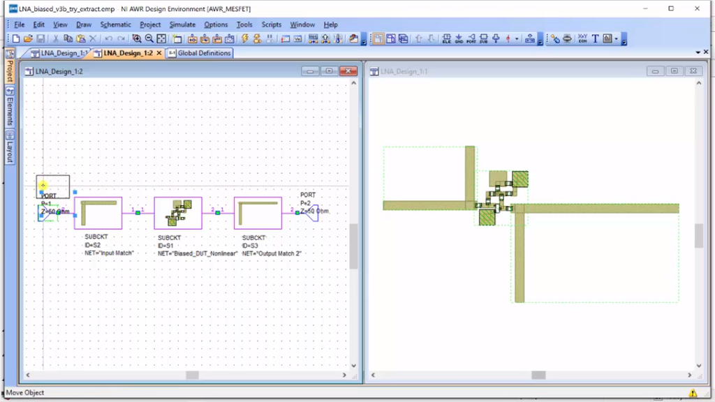
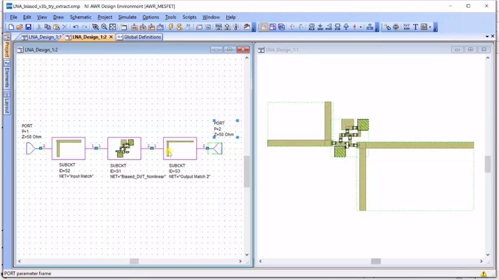
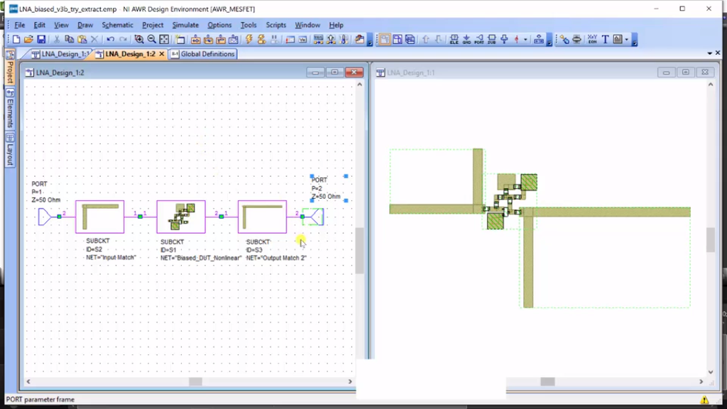
This is a tutorial for using AWR’s iFilter Synthesis Tool to synthesize our impedance for the source and load over RF systems. So, let’s go ahead and talk about why we need synthesized impedance. I’m going to – actually, I’ll move over to an example of a design. So, here we have an amplifier and on the left and right side, we have matching networks that give the load impedance that it needs and the source impedance that it needs. And you’ll notice that the ports on either side are 50 ohms. So, what this network is doing is that it is impedance-matching 50 ohms to what our target impedance is for our source. Here, it’s taking 50 ohms and transforming them into a target impedance for the load. You can look at the tutorials on “Amplifier on Design” to determine what type of impedance is your mainframe amplifier. But, the key thing is we’re looking at the input impedance to this cell and we’re looking at the impedance to this cell because those are equivalent to the load and source impedance on our network.

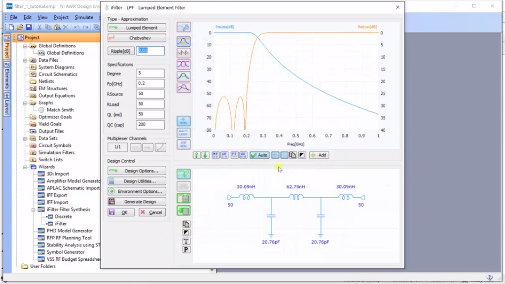
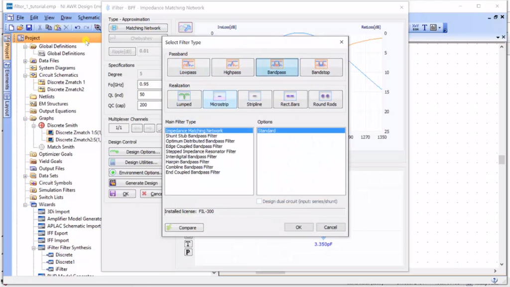
Alright, so let’s go back and try to see if we can synthesize a network. So, I’m going to go to the iFilter Synthesis Tool and typically, it pops off simply as a filter synthesis and if you go under the top, you can choose low-pass, high-pass, or several filters here, or you can choose micro-strip types of filters. But, what is unique is that under the bandpass, I had an extra calculator that really isn’t a filter, but it’s an impedance-matching network and that is what we’re going to use for our impedance matches. So, click “Okay” here, and the idea is it’s going to try to match the impedance on the left to the impedance on the right.

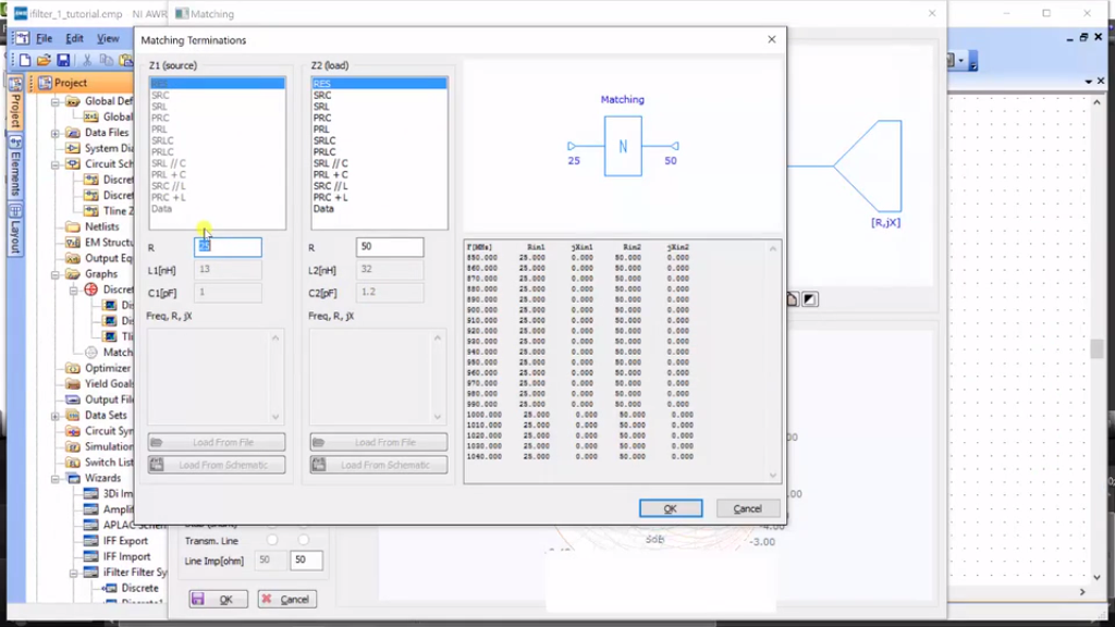
So for the output, let’s just use it. For the load impedance, we’ve got to think about the right being 50 ohms. So, think about this being 50 ohms and we want to write with the impedances looking in from left to right. And so, we set our load as 50 ohms and let’s say that the impedance that we want is 25 + 13 – this is actually in terms of the inductance – 25+ and if you look over here, it’s calculated at 950 is roughly about 77. Now, why do we do this? Well, if you use an RF LC equivalent -by the way, I could just do a “C” here instead- we have a continuous value for X over frequency. If you want to enter in just the real-imaginary part as a point, we could enter in 950, 25, and 100, but this is just a single point, and it’s hard for the synthesis tool to find the optimal around there, whereas if you select a sort of a circuit equivalent for the impedance, it has this ability to get X over a wide range of frequencies and it helps it match better. Alright, so 50 ohms on the right, and the impedance that we would like to see looking into our load is 25 + 75j and the 13 here gives me the 75j right there. So, the impedance at 950 is 25 + 75, and I got that just by going in and changing out to give me the value I want. As you change this, I’ll show you too. You can see that it updates just fine over here and I just find that you can change the value slightly as you go to get the value you need. Alright, hit “Okay”.

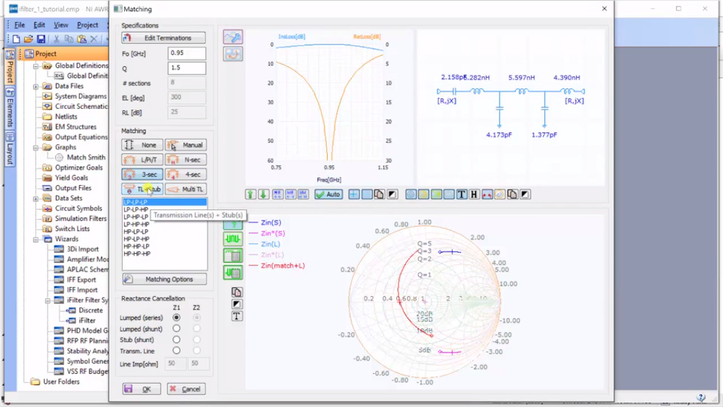
Alright, so there are a lot of impedance matching networks that we can do. There’s the L-pi (L-π), the multi-section, 4-section, and 3-sections; we’ll come back to this one in a second. You can actually do transmission lines, which is super-useful. Alright, so we’re going to click this, and we’re going to do a pi (π) network. It synthesized the network to us. The understanding is that the right is the load and the left is the source, which is defined here. So basically, port 2 is on the right, port 1 is on the left, the right is 50 ohms, and we’ve put in 25 + 13 on the left. Now, we’re going to click “Okay” and we’re almost done. We could choose a real design where we actually put it in, where you can actually see where it’s put in capacitor values with the models, but we don’t actually have these capacitor. So for the sake of simplicity, we’re just going to click “Ideal” and we’re going to click “Generate Design” and I find it useful to deselect everything and the reason is all of this is set up for filters, not for impedance matching network. And I’m going to call this “Discrete Z-Match 1” and I clicked “Okay”. You can see here it created this impedance matching network.

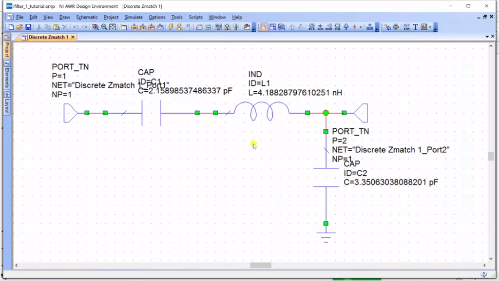
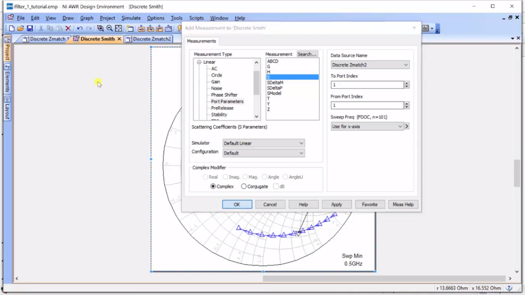
Now, I’ll show you a quick trick. You can go in to AWR and change components just by double-clicking and changing the name. I’m going to change this as a “PORT”, and it immediately sets it to 50 ohms. And I’m going to go over here and do “PORT” and I have 50-ohm here. Now, what I can do is to go to “Projects”, add graph “Discrete Smith”, and this is just going to be the plot of my discrete filter. I create it, add a measurement, and I’m going to do “Discrete Match Z-Match 1”, which is what we have and I click “Okay”, and then I can just run the simulation and now I can add a marker by going into “Graph”, “Marker”, and “Add Marker” and let’s look for 950… There we go.

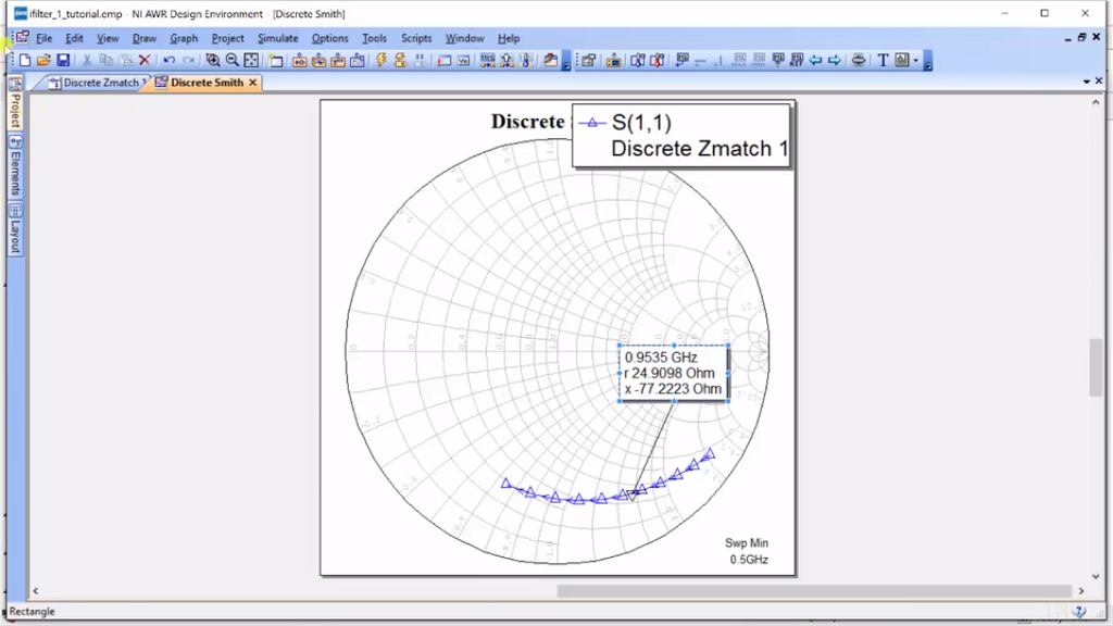
And it’s now giving you R and X in what looks like funky units. And what you do is hit “Options” and you go – it would put it now in before, it was normalizing to 50 ohms, now it’s not. We make sure the real-imaginary and impedance are selected and click “Okay” and there we are. We have 25 – 77j. Now, let’s go back and see what we’ve put in. We go back, and we put in 25 +77. Why did this tool give us -77? Well, this is the “real” part where you have to understand. It gets a little bit confusing. In the impedance matching network, when you put 25 + 13, it would develop the complex conjugate of your source. That is what it means to impedance match. So, what we did is we blindly put the impedance we want and it gave us the complex conjugate of them. That is because this is how the tool works. This is set up not to be Impedance Synthesis but rather Impedance Matching Tool. So, all you have to do is keep in mind that what you put in for targeting impedance should just be the complex conjugate.

So, let’s go to the back and let’s just re-do this. I’m going back through and what I want is 25 -77j because in the matching network will give me 25 + 77. So, I’m just going to “Capacitor” and I’m just going to try to figure out what value it might give me and it takes a little bit of… And we’ll go to… Okay, so here is -77 as my left port. So, this one’s matching network is going to try to look like the complex conjugate. So, it is impedance-looking into it is going to be 25 + 77j around here is 75, 76, and I click “Okay”. I’m already at the pi (π) network, and I click “Okay” again, and generate the design, and “Discrete Z-Match 2”. I’ll just get rid of this…

And here’s my Discrete Z-Match 2 and I’m going in and hit “PORT”, change that to 50 ohms, and go hit that “PORT”, and that’s going to change that to 50 ohms, and then I’m going to my Smith Chart and I could add a new measurement and this would be of Z-Match 2. I’m going to look at S11. And just in case that you’re wondering S11 is because I want to know the impedance looking from the left port in is and why the left port? Just to remind you because that is how I am defining this impedance.

I want this to be 25 + 77j. This is set as 50, and so I’m trying to synthesize the network that takes 50 to 25 +77j. Alright, I’ve done that, so let’s run the simulation. Just click this to move it out of the way. We’re going to add a marker…

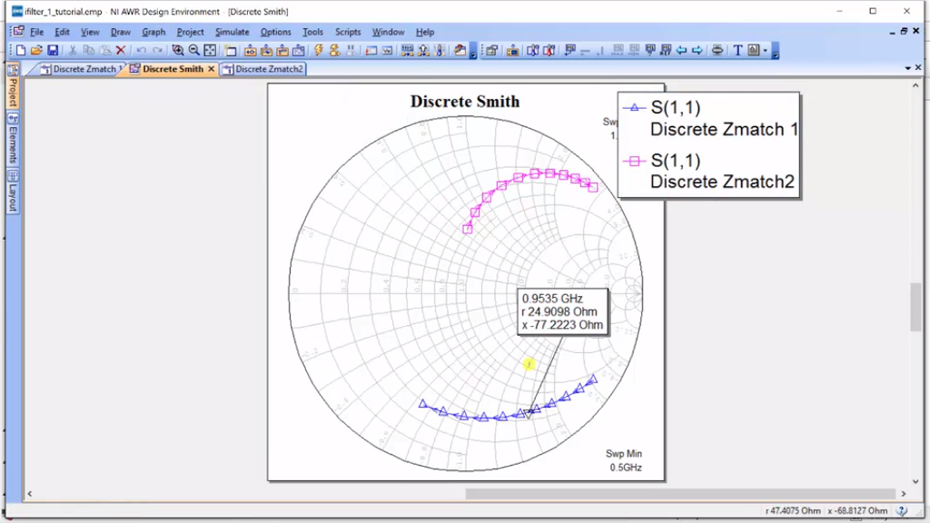
And you can already see it already looks like the complex conjugate and I’m going to go to 950, and ta-da, there we are at 25 + 75j. So, what we have done is we used the Impedance Matching Tool to synthesize the impedance and the only real tricky part is the impedance that you put in for the port you are looking for, which in this case is the source. You need to put in the complex conjugate of it because the complex conjugate is what it would try to create. So, you put the complex conjugate of what you want, the tool will develop a network that creates a complex conjugate of the port and that is what you want. And so, the complex conjugate of the conjugate is what you are looking for.

Alright, so that was as I said for Discrete System, now let’s just go look and see if we wanted to do the same thing, but now let’s do it for the source. And so, we’re looking to the left in, we’re going to terminate with 50 ohms and let’s design a transmission line impedance matching network.

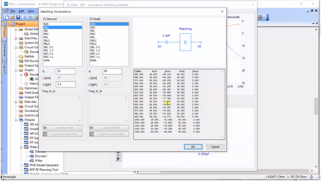
All we do is we go in to iFilter Synthesis; we’re going to the “Matching Network”. Now, you can click “Micro-Strip”. It turns out that later on, we can change this, so we’re not fixed even if you select “Lumped” and I’m going to go ahead and leave this as it is; it’s 50 on the right and I’m sorry; on the left is 50 and it’s all resistive. And on the right, we want it to be 100 and I wanted that to be 25j. So, an inductor would give us 25. You can see here I’m just changing until I can get this down to 25… okay, that is roughly good. So, the port on the right is 100 + 25 and on the left is 50, but hopefully by now you caught my error. What I want is the impedance looking into here to be 100 + 25. So, what I need to do is make this port 100 – 25. So, I clicked on “Src” and I’m going to make this bigger as I go and there we go. It is 25, 26… okay. So now, I’ve put in the complex conjugate because I always had to remember. What I get is 100 + 25, so I enter in 100 – 25 and the network will create an opposite of this, which is what I desire.

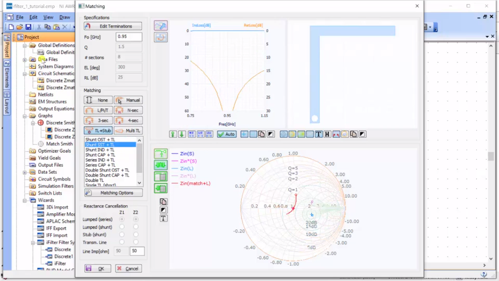
So, click “Okay”, I’ll come back to here, and now, I can click the transmission line stub and it is a whole different bunch of topologies. If you click – Here’s the circuit equivalent or the circuit diagram, you click this and you get the layout. So, these are two transmission lines that are open and for our fabrication technique, that is pretty good. This is a transmission line, but it’s shortened. It’s going to be a lot harder to create shortened transmission lines on fabrication techniques, so I tend to stay away from shortened ones. Here’s one where we have inducted the ground, here’s a capacitor ground, and here’s an inductor in-series and an inductor platform plus a transmission line; we could certainly do that. Here’s a capacitor – I’m sorry, this is a double shunt with two open circuits. Here what I believe is the cap to ground right there and we can do a double transmission line and we could also do a multi-transmission line. We pretty much could do anything that doesn’t require a good short to ground just because of our fabrications. I’m just going to choose this one here and I’m going to click “Okay” and now when I come back to here, this is where we really want to do some new stuff. So, I want to click on “Real” this time because I want to create a real transmission line for us. And I just want to go back to “Matching Network” for a quick second. I’ll show you something.

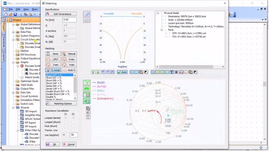
You can go here and this is important because this shows you the dimensions of your transmission line and we probably had it at most 50 or 60 millimeters in any one direction. So, if I looked at this, this is a pretty large design and I could choose a different one to fit within my size. I’ll just go back and look how much this is. So, this is microns. Actually no, it’s pretty good, except 17.8 millimeters by 55.7 millimeters. So, that is a reasonable size. So, it’s good to come down here and check the overall size as well as the layout because you can’t really tell how big this is.

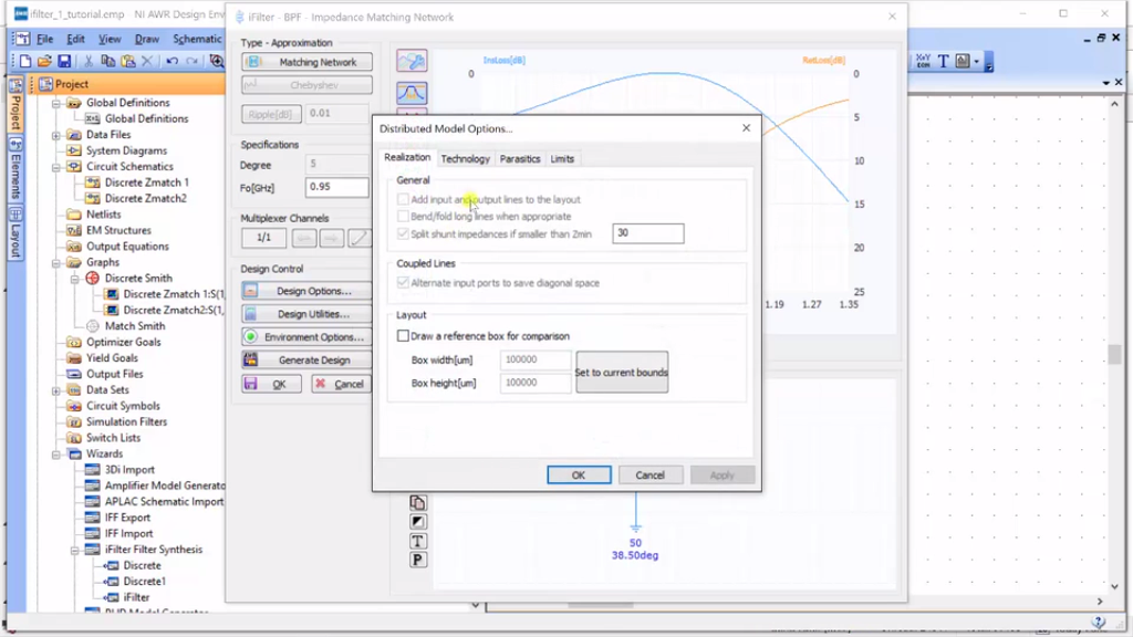
Alright, so we’ve done that, now I’m going to click “Real”, and now I need to go to “Design Options”. So now, here is something that is a little bit annoying. This gooier wizard doesn’t know the stack-up that we used in the design elsewhere. So, we have to put it in ourselves. So for our design, we’re using F for 4, our substrate is 4.5, the height is 5.3 millimeters or 15.30 microns, the conductor thickness is actually 18 microns, and we’ll just make something that is not too – the load is there, and I click “Okay”. We’re ready to go and I click “Real” and I’m going to generate the design and I’m going to put “Tline Zmatch 1”. Now, I’ll close out of this.

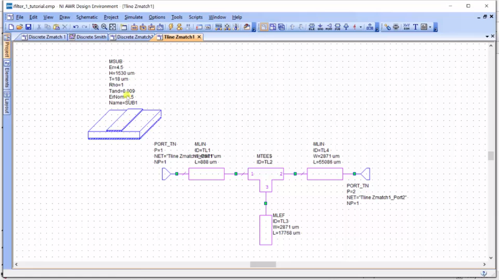
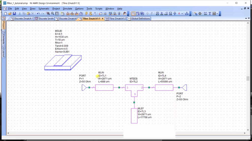
Now, look at what it has done. It’s put in a MSUB, based upon what we’ve added, but for our work, we already had an MSUB Global Definition. So, we’re actually going to disable this, but you can see that it has the height, the thickness, and everything that’s there. And these are actually micro-strip transmission lines. You can see – I’ll move this out of the way – You can see one length, you can see the other length, we put in a T, we did the entire design for you, and if you wanted to, you can click right here and view layout, like that. We’ve got this great transmission line. I’m going to do just what I did before. I’m going to change this one to 50 ohms. So, this is port and I’m going to change this one to port. And remember, S22 is looking in from the right to the left and that is where we wanted to learn here from the right to the left. And so, I can go ahead and add it to my Smith Chart here just because it says “Discrete” doesn’t mean I can’t add it. I’ll add in a new measurement from the TZmatch and I want to do S22 and I click “Okay”.

Alright, so here we are. We’ve created Z22. I’ll move this out of the way and I’m going to add a marker and here. You can see 950 that I have roughly. You can see the change very quickly 100 + 10j. So, if I put a marker here at 95, you can see that I have 100 + 17j, which is pretty close to the 100 + 25j that I was looking for. It is a little bit off, but it is pretty close. You can see that we can synthesize the impedance with the transmission line and what is nice is that we actually have the layout now and so, we can create our design with our layout directly from this schematic.

Now, I just want to show you one last thing that might confuse you because the iWizard tool is not perfect in every way. Let’s go back to this slide where we wanted the impedance looking in at 25 + 72j and let’s try to synthesize that with transmission lines. I could go to iFilter Synthesis, Matching Networks, select this, and I’m just going to click “Okay” here because I want to select that I’m going to do a transmission line and you noticed what happened here. It’s telling me that my source must be resistive.

Okay, let’s go back… When you are doing a transmission line, the left side always has to be resistive. Now, that can be a little bit confusing because we would like the right side to be resistive and the left side to be the complex impedance that we’re trying to do, but that’s no worries. We can just view this as flipped around. So basically, what we are going to do is if you will, I’m just going to move this, I’ll delete this and this is just for our clarity, we’re going to design this. Think of it this way as the left being 50 ohms and the impedance looking in is going to be 25 + 75j. That is how we are going to design it with the iFilter tool and all we need to remember is that we need to connect to this port 1 – I’m sorry, we need to connect the right-hand port, which in the case of the matching network, will be port 2 to this node. So, let’s just do that real quick. I’ll show you.

So, the source is 50 ohms and then, we want this to be 25 and we need to do the complex conjugate. So, I need to choose a capacitor to get negative. Alright, there we are at 77 roughly, okay. Click “Okay” and I’m going to look at the layout. That is what it looks like. The size is 31 by 38 millimeters and that’s okay. And then, I’m going to hit the “Design Options” to make sure my substrate looks right and it does. Actually, it’s a little bit off. So, I’ll just tune this here. Click “Okay” and then I will generate the design and I will call this “Tline Zmatch 3” and I’m not sure if I had “2”, but if I did, that’s alright, and I click “Okay” and there we are. So, here’s our design and I hit port and I’m going to hit port.

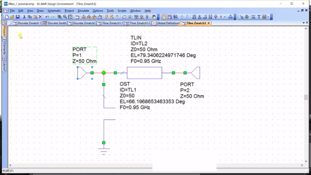
Alright, remember for the iWizard, the left half had to be 50 ohms and we design the right half to be 25 + 77j, but this is port 2. So, when we go put this on a schematic, I will go ahead and do a new schematic and we go to “Elements” and we go to “Sub-Circuits” and we would go to “Tline Zmatch 3” and let’s just put this in right there.

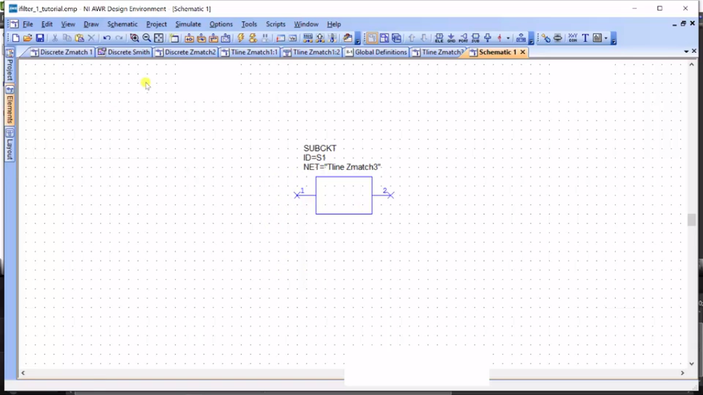
This is Tline Zmatch 3. Remember, the left one is the one we matched to 50 ohms. So, we have to select it, rotate it, support 1 is on the right, and now I will connect it up. That is “Port 1”, that is “Port 2” and let’s just do a new graph for this. We’ll do a Smith Chart and I will add a measurement of – and remember that this is a schematic and it’s “Schematic 1” and “Port 22” and why are we doing 22 because we want to look from the left to the right in and I’ll hit this here, there we go, and I will then do a graph and a marker…

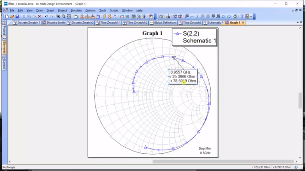
And there we are. As you can see, it is 25 plus roughly 77j. Alright, so the key thing to remember here is that we had a flip this around because the left side of the iFilter tool, I’ll just go back one last time… Matching network, okay… The left side for transmission lines needs to be 50 ohms and when it synthesizes it; the left side is always going to be port 1. So, if you’re in a situation like this, where you need to look into the right, what you need to do is flipping this around so that the left port is 50 and the right port is what you synthesize. It’s not too hard. You can see that we can keep track of the port definitions for the synthesis tool. Alright, give it a try. This is a great way to design impedance matching networks with the iMatch tool.